In this tutorial, we will build a hierarchical acausal component-based model of the RC circuit. The RC circuit is a simple example where we connect a resistor and a capacitor. Kirchhoff's laws are then applied to state equalities between currents and voltages. This specifies a differential-algebraic equation (DAE) system, where the algebraic equations are given by the constraints and equalities between different component variables. We then simplify this to an ODE by eliminating the equalities before solving. Let's see this in action.
!!! note
This tutorial teaches how to build the entire RC circuit from scratch.
However, to simulate electric components with more ease, check out the
[ModelingToolkitStandardLibrary.jl](https://docs.sciml.ai/ModelingToolkitStandardLibrary/stable/)
which includes a
[tutorial for simulating RC circuits with pre-built components](https://docs.sciml.ai/ModelingToolkitStandardLibrary/stable/tutorials/rc_circuit/)
using ModelingToolkit, Plots, OrdinaryDiffEq
using ModelingToolkit: t_nounits as t, D_nounits as D

@connector Pin begin
    v(t)
    i(t), [connect = Flow]
end

@mtkmodel Ground begin
    @components begin
        g = Pin()
    end
    @equations begin
        g.v ~ 0
    end
end

@mtkmodel OnePort begin
    @components begin
        p = Pin()
        n = Pin()
    end
    @variables begin
        v(t)
        i(t)
    end
    @equations begin
        v ~ p.v - n.v
        0 ~ p.i + n.i
        i ~ p.i
    end
end

@mtkmodel Resistor begin
    @extend OnePort()
    @parameters begin
        R = 1.0 # Sets the default resistance
    end
    @equations begin
        v ~ i * R
    end
end

@mtkmodel Capacitor begin
    @extend OnePort()
    @parameters begin
        C = 1.0
    end
    @equations begin
        D(v) ~ i / C
    end
end

@mtkmodel ConstantVoltage begin
    @extend OnePort()
    @parameters begin
        V = 1.0
    end
    @equations begin
        V ~ v
    end
end

@mtkmodel RCModel begin
    @description "A circuit with a constant voltage source, resistor and capacitor connected in series."
    @components begin
        resistor = Resistor(R = 1.0)
        capacitor = Capacitor(C = 1.0)
        source = ConstantVoltage(V = 1.0)
        ground = Ground()
    end
    @equations begin
        connect(source.p, resistor.p)
        connect(resistor.n, capacitor.p)
        connect(capacitor.n, source.n)
        connect(capacitor.n, ground.g)
    end
end

@mtkbuild rc_model = RCModel(resistor.R = 2.0)
u0 = [
    rc_model.capacitor.v => 0.0
]
prob = ODEProblem(rc_model, u0, (0, 10.0))
sol = solve(prob)
plot(sol)
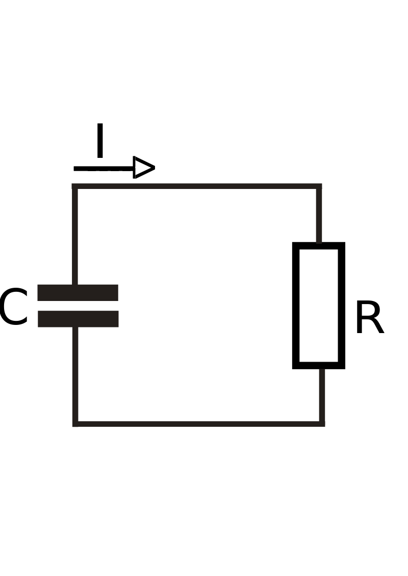
We wish to build the following RC circuit by building individual components and connecting the pins:
For each of our components, we use ModelingToolkit Model that emits an ODESystem.
At the top, we start with defining the fundamental qualities of an electric
circuit component. At every input and output pin, a circuit component has
two values: the current at the pin and the voltage. Thus we define the Pin
component (connector) to simply be the values there. Whenever two Pins in a
circuit are connected together, the system satisfies Kirchhoff's laws,
i.e. that currents sum to zero and voltages across the pins are equal.
[connect = Flow] informs MTK that currents ought to sum to zero, and by
default, variables are equal in a connection.
@connector Pin begin
    v(t)
    i(t), [connect = Flow]
end
Note that this is an incompletely specified ODESystem: it cannot be simulated
on its own because the equations for v(t) and i(t) are unknown. Instead,
this just gives a common syntax for receiving this pair with some default
values.
One can then construct a Pin using the @named helper macro:
@named mypin1 = Pin()
Next, we build our ground node. A ground node is just a pin that is connected
to a constant voltage reservoir, typically taken to be V = 0. Thus to define
this component, we generate an ODESystem with a Pin subcomponent and specify
that the voltage in such a Pin is equal to zero. This gives:
@mtkmodel Ground begin
    @components begin
        g = Pin()
    end
    @equations begin
        g.v ~ 0
    end
end
Next we build a OnePort: an abstraction for all simple electric component
with two pins. The voltage difference between the positive pin and the negative
pin is the voltage of the component, the current between two pins must sum to
zero, and the current of the component equals to the current of the positive
pin.
@mtkmodel OnePort begin
    @components begin
        p = Pin()
        n = Pin()
    end
    @variables begin
        v(t)
        i(t)
    end
    @equations begin
        v ~ p.v - n.v
        0 ~ p.i + n.i
        i ~ p.i
    end
end
Next we build a resistor. A resistor is an object that has two Pins, the positive
and the negative pins, and follows Ohm's law: v = i*r. The voltage of the
resistor is given as the voltage difference across the two pins, while by conservation
of charge we know that the current in must equal the current out, which means
(no matter the direction of the current flow) the sum of the currents must be
zero. This leads to our resistor equations:
@mtkmodel Resistor begin
    @extend OnePort()
    @parameters begin
        R = 1.0
    end
    @equations begin
        v ~ i * R
    end
end
Notice that we have created this system with a default parameter R for the
resistor's resistance. By doing so, if the resistance of this resistor is not
overridden by a higher level default or overridden at ODEProblem construction
time, this will be the value of the resistance. Also, note the use of @extend.
For the Resistor, we want to simply inherit OnePort's
equations and unknowns and extend them with a new equation. Note that v, i are not namespaced as oneport.v or oneport.i.
Using our knowledge of circuits, we similarly construct the Capacitor:
@mtkmodel Capacitor begin
    @extend OnePort()
    @parameters begin
        C = 1.0
    end
    @equations begin
        D(v) ~ i / C
    end
end
Now we want to build a constant voltage electric source term. We can think of this as similarly being a two pin object, where the object itself is kept at a constant voltage, essentially generating the electric current. We would then model this as:
@mtkmodel ConstantVoltage begin
    @extend OnePort()
    @parameters begin
        V = 1.0
    end
    @equations begin
        V ~ v
    end
end
Note that as we are extending only v from OnePort, it is explicitly specified as a tuple.
Now we are ready to simulate our circuit. Let's build our four components:
a resistor, capacitor, source, and ground term. For simplicity, we will
make all of our parameter values 1.0. As resistor, capacitor, source lists
R, C, V in their argument list, they are promoted as arguments of RCModel as
resistor.R, capacitor.C, source.V
@mtkmodel RCModel begin
    @description "A circuit with a constant voltage source, resistor and capacitor connected in series."
    @components begin
        resistor = Resistor(R = 1.0)
        capacitor = Capacitor(C = 1.0)
        source = ConstantVoltage(V = 1.0)
        ground = Ground()
    end
    @equations begin
        connect(source.p, resistor.p)
        connect(resistor.n, capacitor.p)
        connect(capacitor.n, source.n)
        connect(capacitor.n, ground.g)
    end
end
We can create a RCModel component with @named. And using subcomponent_name.parameter we can set
the parameters or defaults values of variables of subcomponents.
@mtkbuild rc_model = RCModel(resistor.R = 2.0)
This model is acausal because we have not specified anything about the causality of the model. We have simply specified what is true about each of the variables. This forms a system of differential-algebraic equations (DAEs) which define the evolution of each unknown of the system. The equations are:
equations(expand_connections(rc_model))
the unknowns are:
unknowns(rc_model)
and the parameters are:
parameters(rc_model)
The observed equations are:
observed(rc_model)
We are left with a system of only two equations with two unknown variables. One of the equations is a differential equation, while the other is an algebraic equation. We can then give the values for the initial conditions of our unknowns, and solve the system by converting it to an ODEProblem in mass matrix form and solving it with an ODEProblem mass matrix DAE solver. This is done as follows:
u0 = [rc_model.capacitor.v => 0.0]

prob = ODEProblem(rc_model, u0, (0, 10.0))
sol = solve(prob)
plot(sol)
However, what if we wanted to plot the timeseries of a different variable? Do
not worry, that information was not thrown away! Instead, transformations
like structural_simplify simply change unknown variables into observables which are
defined by observed equations.
observed(rc_model)
These are explicit algebraic equations which can then be used to reconstruct the required variables on the fly. This leads to dramatic computational savings because implicitly solving an ODE scales like O(n^3), so making there be as few unknowns as possible is good!
The solution object can be accessed via its symbols. For example, let's retrieve the voltage of the resistor over time:
sol[rc_model.resistor.v]
or we can plot the timeseries of the resistor's voltage:
plot(sol, idxs = [rc_model.resistor.v])