This repository provides scripts and recipes to train EfficientNet v1-B0 and v1-B4 to achieve state-of-the-art accuracy. The content of the repository is maintained by NVIDIA and is tested against each NGC monthly released container to ensure consistent accuracy and performance over time.
-
- Benchmarking
- Training performance benchmark
- Results
- Training accuracy results for EfficientNet v1-B0
- Training accuracy results for EfficientNet v1-B4
- Training performance results for EfficientNet v1-B0
- Training performance results for EfficientNet v1-B4
- Inference performance results for EfficientNet v1-B0
- Inference performance results for EfficientNet v1-B4
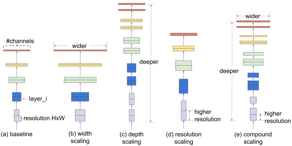
EfficientNet v1 is developed based on AutoML and Compound Scaling. In particular, a mobile-size baseline network called EfficientNet v1-B0 is developed from AutoML MNAS Mobile framework, the building block is mobile inverted bottleneck MBConv with squeeze-and-excitation optimization. Then, through a compound scaling method, this baseline is scaled up to obtain EfficientNet v1-B1 to B7.
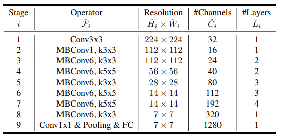
Here is the Baseline EfficientNet v1-B0 structure.
The following features are supported by this implementation:
-
General:
- XLA support
- Mixed precision support
- Multi-GPU support using Horovod
- Multi-node support using Horovod
- Cosine LR Decay
-
Inference:
- Support for inference on a single image is included
- Support for inference on a batch of images is included
| Feature | EfficientNet |
|---|---|
| Horovod Multi-GPU training (NCCL) | Yes |
| Multi-GPU training | Yes |
| Multi-node training | Yes |
| Automatic mixed precision (AMP) | Yes |
| XLA | Yes |
| Gradient Accumulation | Yes |
| Stage-wise Training | Yes |
Multi-GPU training with Horovod
Our model uses Horovod to implement efficient multi-GPU training with NCCL. For details, refer to example sources in this repository or refer to the TensorFlow tutorial.
Multi-node training with Horovod
Our model also uses Horovod to implement efficient multi-node training.
Automatic Mixed Precision (AMP)
Computation graphs can be modified by TensorFlow on runtime to support mixed precision training. A detailed explanation of mixed precision can be found in Appendix.
Gradient Accumulation
Gradient Accumulation is supported through a custom train_step function. This feature is enabled only when grad_accum_steps is greater than 1.
Mixed precision is the combined use of different numerical precisions in a computational method. Mixed precision training offers significant computational speedup by performing operations in half-precision format while storing minimal information in single-precision to retain as much information as possible in critical parts of the network. Since the introduction of Tensor Cores in NVIDIA Volta, and following with both the NVIDIA Turing and NVIDIA Ampere architectures, significant training speedups are experienced by switching to mixed precision -- up to 3x overall speedup on the most arithmetically intense model architectures. Using mixed precision training previously required two steps:
- Porting the model to use the FP16 data type where appropriate.
- Adding loss scaling to preserve small gradient values.
This can now be achieved using Automatic Mixed Precision (AMP) for TensorFlow to enable the full mixed precision methodology in your existing TensorFlow model code. AMP enables mixed precision training on NVIDIA Volta, NVIDIA Turing, and NVIDIA Ampere GPU architectures automatically. The TensorFlow framework code makes all necessary model changes internally.
In TF-AMP, the computational graph is optimized to use as few casts as necessary and maximize the use of FP16, and the loss scaling is automatically applied inside of supported optimizers. AMP can be configured to work with the existing tf.contrib loss scaling manager by disabling the AMP scaling with a single environment variable to perform only the automatic mixed-precision optimization. It accomplishes this by automatically rewriting all computation graphs with the necessary operations to enable mixed precision training and automatic loss scaling.
For information about:
- How to train using mixed precision, refer to the Mixed Precision Training paper and Training With Mixed Precision documentation.
- Techniques used for mixed precision training, refer to the Mixed-Precision Training of Deep Neural Networks blog.
- How to access and enable AMP for TensorFlow, refer to Using TF-AMP from the TensorFlow User Guide.
Mixed precision is enabled in TensorFlow by using the Automatic Mixed Precision (TF-AMP) extension, which casts variables to half-precision upon retrieval while storing variables in single-precision format. Furthermore, to preserve small gradient magnitudes in backpropagation, a loss scaling step must be included when applying gradients. In TensorFlow, loss scaling can be applied statically by using simple multiplication of loss by a constant value or automatically, by TF-AMP. Automatic mixed precision makes all the adjustments internally in TensorFlow, providing two benefits over manual operations. First, programmers need not modify network model code, reducing development and maintenance effort. Second, using AMP maintains forward and backward compatibility with all the APIs for defining and running TensorFlow models.
To enable mixed precision, you can simply add the --use_amp to the command-line used to run the model. This will enable the following code:
if params.use_amp:
    policy = tf.keras.mixed_precision.experimental.Policy('mixed_float16', loss_scale='dynamic')
    tf.keras.mixed_precision.experimental.set_policy(policy)
TensorFloat-32 (TF32) is the new math mode in NVIDIA A100 GPUs for handling the matrix math, also called tensor operations. TF32 running on Tensor Cores in A100 GPUs can provide up to 10x speedups compared to single-precision floating-point math (FP32) on NVIDIA Volta GPUs.
TF32 Tensor Cores can speed up networks using FP32, typically with no loss of accuracy. It is more robust than FP16 for models which require a high dynamic range for weights or activations.
For more information, refer to the TensorFloat-32 in the A100 GPU Accelerates AI Training, HPC up to 20x blog post.
TF32 is supported in the NVIDIA Ampere GPU architecture and is enabled by default.
The following section lists the requirements that you need to meet in order to start training the EfficientNet model.
This repository contains Dockerfile which extends the TensorFlow NGC container and encapsulates some dependencies. Aside from these dependencies, ensure you have the following components:
- NVIDIA Docker
- [TensorFlow 21.09-py3] NGC container or later
- Supported GPUs:
For more information about how to get started with NGC containers, refer to the following sections from the NVIDIA GPU Cloud Documentation and the Deep Learning Documentation:
- Getting Started Using NVIDIA GPU Cloud
- Accessing And Pulling From The NGC Container Registry
- Running TensorFlow
As an alternative to the use of the Tensorflow2 NGC container, to set up the required environment or create your own container, refer to the versioned NVIDIA Container Support Matrix.
For multi-node, the sample provided in this repository requires Enroot and Pyxis set up on a SLURM cluster.
To train your model using mixed or TF32 precision with Tensor Cores or using FP32, perform the following steps using the default parameters of the EfficientNet model on the ImageNet dataset. For the specifics concerning training and inference, refer to the Advanced section.
-
Clone the repository.
git clone https://github.com/NVIDIA/DeepLearningExamples.git cd DeepLearningExamples/TensorFlow2/Classification/ConvNets/efficientnet -
Download and prepare the dataset.
Runner.pysupports ImageNet with TensorFlow Datasets (TFDS). Refer to the TFDS ImageNet readme for manual download instructions. -
Build EfficientNet on top of the NGC container.
bash ./scripts/docker/build.sh YOUR_DESIRED_CONTAINER_NAME -
Start an interactive session in the NGC container to run training/inference. Ensure that
launch.shhas the correct path to ImageNet on your machine and that this path is mounted onto the/datadirectory because this is where training and evaluation scripts search for data.`bash ./scripts/docker/launch.sh YOUR_DESIRED_CONTAINER_NAME` -
Start training.
To run training for a standard configuration, under the container default entry point
/workspace, run one of the scripts in the./efficinetnet_v1/{B0,B4}/training/{AMP,TF32,FP32}/convergence_8x{A100-80G, V100-32G}.sh. For example:bash ./efficinetnet_v1/B0/training/AMP/convergence_8xA100-80G.sh -
Start validation/evaluation.
To run validation/evaluation for a standard configuration, under the container default entry point
/workspace, run one of the scripts in the./efficinetnet_v1/{B0,B4}/evaluation/evaluation_{AMP,FP32,TF32}_8x{A100-80G, V100-32G}.sh. The evaluation script is configured to use the checkpoint specified incheckpointfor evaluation. The specified checkpoint will be read from the location passed by `--model_dir'.For example:bash ./efficinetnet_v1/B0/evaluation/evaluation_AMP_A100-80G.sh -
Start inference/predictions.
To run inference for a standard configuration, under the container default entry point
/workspace, run one of the scripts in the./efficinetnet_v1/{B0,B4}/inference/inference_{AMP,FP32,TF32}.sh. Ensure your JPEG images used to run inference on are mounted in the/infer_datadirectory with this folder structure :infer_data | ├── images | | ├── image1.JPEG | | ├── image2.JPEGFor example:
bash ./efficinetnet_v1/B0/inference/inference_AMP.sh
Now that you have your model trained and evaluated, you can choose to compare your training results with our Training accuracy results. You can also choose to benchmark your performance to Training performance benchmark or Inference performance benchmark. Following the steps in these sections will ensure that you achieve the same accuracy and performance results as stated in the Results section.
The following sections provide greater details of the dataset, running training and inference, and the training results.
The repository is structured as follows:
scripts/- shell scripts to build and launch EfficientNet container on top of NGC containerefficientnet_{v1,v2}scripts to launch training, evaluation and inferencemodel/- building blocks and EfficientNet model definitionsruntime/- detailed procedure for each running modeutils/- support util functions for learning rates, optimizers, etc.dataloader/provides data pipeline utilsconfig/contains model definitions
The hyper parameters can be grouped into model-specific hyperparameters (e.g., #layers ) and general hyperparameters (e.g., #training epochs).
The model-specific hyperparameters are to be defined in a python module, which must be passed in the command line via --cfg ( python main.py --cfg config/efficientnet_v1/b0_cfg.py). To override model-specific hyperparameters, you can use a comma-separated list of k=v pairs (e.g., python main.py --cfg config/efficientnet_v1/b0_cfg.py --mparams=bn_momentum=0.9,dropout=0.5).
The general hyperparameters and their default values can be found in utils/cmdline_helper.py. The user can override these hyperparameters in the command line (e.g., python main.py --cfg config/efficientnet_v1/b0_cfg.py --data_dir xx --train_batch_size 128). Here is a list of important hyperparameters:
-
--mode(train_and_eval,train,eval,prediction) - the default istrain_and_eval. -
--use_ampSet to True to enable AMP -
--use_xlaSet to True to enable XLA -
--model_dirThe folder where model checkpoints are saved (the default is/workspace/output) -
--data_dirThe folder where data resides (the default is/data/) -
--log_stepsThe interval of steps between logging of batch level stats. -
--augmenter_nameType of data augmentation -
--raug_num_layersNumber of layers used in the random data augmentation scheme -
--raug_magnitudeStrength of transformations applied in the random data augmentation scheme -
--cutmix_alphaCutmix parameter used in the last stage of training. -
--mixup_alphaMixup parameter used in the last stage of training. -
--defer_img_mixingMove image mixing ops from the data loader to the model/GPU (faster training) -
--eval_img_sizeSize of images used for evaluation -
--eval_batch_sizeThe evaluation batch size per GPU -
--n_stagesNumber of stages used for stage-wise training -
--train_batch_sizeThe training batch size per GPU -
--train_img_sizeSize of images used in the last stage of training -
--base_img_sizeSize of images used in the first stage of training -
--max_epochsThe number of training epochs -
--warmup_epochsThe number of epochs of warmup -
--moving_average_decayThe decay weight used for EMA -
--lr_initThe learning rate for a batch size of 128, effective learning rate will be automatically scaled according to the global training batch size:lr=lr_init * global_BS/128 where global_BS=train_batch_size*n_GPUs -
--lr_decayLearning rate decay policy -
--weight_decayWeight decay coefficient -
--save_checkpoint_freqNumber of epochs to save checkpoints
NOTE: Avoid changing the default values of the general hyperparameters provided in utils/cmdline_helper.py. The reason is that some other models supported by this repository may rely on such default values. If you want to change the values, override them via the command line.
To display the full list of available options and their descriptions, use the -h or --help command-line option, for example:
python main.py --help
Refer to the TFDS ImageNet readme for manual download instructions.
To train on the ImageNet dataset, pass $path_to_ImageNet_tfrecords to $data_dir in the command-line.
Name the TFRecords in the following scheme:
- Training images -
/data/train-* - Validation images -
/data/validation-*
The training process can start from scratch or resume from a checkpoint.
By default, bash script scripts/{B0,B4}/training/{AMP,FP32,TF32}/convergence_8x{A100-80G,V100-32G}.sh will start the training process with the following settings.
- Use 8 GPUs by Horovod
- Has XLA enabled
- Saves checkpoints after every 10 epochs to
/workspace/output/folder - AMP or FP32 or TF32 based on the folder
scripts/{B0,B4}/training/{AMP, FP32, TF32}
The training starts from scratch if --model_dir has no checkpoints in it. To resume from a checkpoint, place the checkpoint into --model_dir and make sure the checkpoint file points to it.
Multi-node runs can be launched on a Pyxis/enroot Slurm cluster (refer to Requirements) with the run_{B0,B4}_multinode.sub script with the following command for a 4-node NVIDIA DGX A100 example:
PARTITION=<partition_name> sbatch N 4 --ntasks-per-node=8 run_B0_multinode.sub
PARTITION=<partition_name> sbatch N 4 --ntasks-per-node=8 run_B4_multinode.sub
Checkpoints will be saved after --save_checkpoint_freq epochs at checkpointdir. The latest checkpoint will be automatically picked up to resume training in case it needs to be resumed. Cluster partition name has to be provided <partition_name>.
Note that the run_{B0,B4}_multinode.sub script is a starting point that has to be adapted depending on the environment. In particular, pay attention to the variables such as --container-image, which handles the container image to train, and --datadir, which handles the location of the ImageNet data.
Refer to the scripts to find the full list of variables to adjust for your system.
Validation can be done either during training (when --mode train_and_eval is used) or in a post-training setting (--mode eval) on a checkpointed model. The evaluation script expects data in the tfrecord format.
bash ./scripts/{B0,B4}/evaluation/evaluation_{AMP,FP32,TF32}_{A100-80G,V100-32G}.sh
Metrics gathered through this process are as follows:
- eval_loss
- eval_accuracy_top_1
- eval_accuracy_top_5
- avg_exp_per_second_eval
- avg_exp_per_second_eval_per_GPU
- avg_time_per_exp_eval : Average Latency
- latency_90pct : 90% Latency
- latency_95pct : 95% Latency
- latency_99pct : 99% Latency
The scripts used for inference expect the inference data in the following directory structure:
```
infer_data
|   ├── images
|   |   ├── image1.JPEG
|   |   ├── image2.JPEG
```
Run:
bash ./scripts/{B0,B4}/inference/inference_{AMP,FP32,TF32}.sh
The performance measurements in this document were conducted at the time of publication and may not reflect the performance achieved from NVIDIA’s latest software release. For the most up-to-date performance measurements, go to NVIDIA Data Center Deep Learning Product Performance.
The following section shows how to run benchmarks measuring the model performance in training and inference modes.
Training benchmark for EfficientNet v1-B0 was run on NVIDIA DGX A100 80GB and NVIDIA DGX-1 V100 32GB.
To benchmark training performance with other parameters, run:
bash ./scripts/B0/training/{AMP, FP32, TF32}/train_benchmark_8x{A100-80G, V100-32G}.sh
Training benchmark for EfficientNet v1-B4 was run on NVIDIA DGX A100 80GB and NVIDIA DGX-1 V100 32GB.
bash ./scripts/B4/training/{AMP, FP32, TF32}/train_benchmark_8x{A100-80G, V100-32G}.sh
Inference benchmark for EfficientNet v1-B0 was run on NVIDIA DGX A100 80GB and NVIDIA DGX-1 V100 32GB.
Inference benchmark for EfficientNet v1-B4 was run on NVIDIA DGX A100 80GB and NVIDIA DGX-1 V100 32GB.
The following sections provide details on how we achieved our performance and accuracy in training and inference.
Our results were obtained by running the training scripts in the tensorflow:21.09-tf2-py3 NGC container on NVIDIA DGX A100 (8x A100 80GB) GPUs. We evaluated the models using both the original and EMA weights and selected the higher accuracy to report.
| GPUs | Accuracy - TF32 | Accuracy - mixed precision | Time to train - TF32 | Time to train - mixed precision | Time to train speedup (TF32 to mixed precision) |
|---|---|---|---|---|---|
| 8 | 77.60% | 77.59% | 19.5hrs | 8.5hrs | 2.29 |
| 16 | 77.51% | 77.48% | 10hrs | 4.5hrs | 2.22 |
Our results were obtained by running the training scripts in the tensorflow:21.09-tf2-py3 NGC container on NVIDIA DGX V100 (8x V100 32GB) GPUs. We evaluated the models using both the original and EMA weights and selected the higher accuracy to report.
| GPUs | Accuracy - FP32 | Accuracy - mixed precision | Time to train - FP32 | Time to train - mixed precision | Time to train speedup (FP32 to mixed precision) |
|---|---|---|---|---|---|
| 8 | 77.67% | 77.69% | 49.0hrs | 38.0hrs | 1.29 |
| 32 | 77.55% | 77.53% | 11.5hrs | 10hrs | 1.15 |
Our results were obtained by running the training scripts in the tensorflow:21.09-tf2-py3 NGC container on multi-node NVIDIA DGX A100 (8x A100 80GB) GPUs. We evaluated the models using both the original and EMA weights and selected the higher accuracy to report.
| GPUs | Accuracy - TF32 | Accuracy - mixed precision | Time to train - TF32 | Time to train - mixed precision | Time to train speedup (TF32 to mixed precision) |
|---|---|---|---|---|---|
| 32 | 82.98% | 83.13% | 38hrs | 14hrs | 2.00 |
| 64 | 83.14% | 83.05% | 19hrs | 7hrs | 2.00 |
Our results were obtained by running the training scripts in the tensorflow:21.09-tf2-py3 NGC container on NVIDIA DGX V100 (8x A100 32GB) GPUs. We evaluated the models using both the original and EMA weights and selected the higher accuracy to report.
| GPUs | Accuracy - FP32 | Accuracy - mixed precision | Time to train - TF32 | Time to train - mixed precision | Time to train speedup (FP32 to mixed precision) |
|---|---|---|---|---|---|
| 32 | 82.64% | 82.88% | 97.0hrs | 41.0hrs | 2.37 |
| 64 | 82.74% | 83.16% | 50.0hrs | 20.5hrs | 2.43 |
| GPUs | Throughput - TF32 | Throughput - mixed precision | Throughput speedup (TF32 - mixed precision) | Weak scaling - TF32 | Weak scaling - mixed precision |
|---|---|---|---|---|---|
| 1 | 1209 | 3454 | 2.85 | 1 | 1 |
| 8 | 9119 | 20647 | 2.26 | 7.54 | 5.98 |
| 16 | 17815 | 40644 | 2.28 | 14.74 | 11.77 |
| GPUs | Throughput - FP32 | Throughput - mixed precision | Throughput speedup (FP32 - mixed precision) | Weak scaling - FP32 | Weak scaling - mixed precision |
|---|---|---|---|---|---|
| 1 | 752 | 868 | 1.15 | 1 | 1 |
| 8 | 4504 | 4880 | 1.08 | 5.99 | 5.62 |
| 32 | 15309 | 18424 | 1.20 | 20.36 | 21.23 |
| GPUs | Throughput - TF32 | Throughput - mixed precision | Throughput speedup (TF32 - mixed precision) | Weak scaling - TF32 | Weak scaling - mixed precision |
|---|---|---|---|---|---|
| 1 | 165 | 470 | 2.85 | 1 | 1 |
| 8 | 1308 | 3550 | 2.71 | 7.93 | 7.55 |
| 32 | 4782 | 12908 | 2.70 | 28.98 | 27.46 |
| 64 | 9473 | 25455 | 2.69 | 57.41 | 54.16 |
| GPUs | Throughput - FP32 | Throughput - mixed precision | Throughput speedup (FP32 - mixed precision) | Weak scaling - TF32 | Weak scaling - mixed precision |
|---|---|---|---|---|---|
| 1 | 79 | 211 | 2.67 | 1 | 1 |
| 8 | 570 | 1258 | 2.21 | 7.22 | 5.96 |
| 32 | 1855 | 4325 | 2.33 | 23.48 | 20.50 |
| 64 | 3568 | 8643 | 2.42 | 45.16 | 40.96 |
Our results were obtained by running the inferencing benchmarking script in the tensorflow:21.09-tf2-py3 NGC container on the NVIDIA DGX A100 (1x A100 80GB) GPU.
FP16 Inference Latency
| Batch size | Resolution | Throughput Avg | Latency Avg (ms) | Latency 90% (ms) | Latency 95% (ms) | Latency 99% (ms) |
|---|---|---|---|---|---|---|
| 1 | 224x224 | 110.97 | 9.09 | 9.02 | 9.04 | 9.09 |
| 8 | 224x224 | 874.91 | 9.12 | 9.04 | 9.08 | 9.12 |
| 32 | 224x224 | 2188.84 | 14.62 | 14.35 | 14.43 | 14.52 |
| 1024 | 224x224 | 9729.85 | 105.24 | 101.50 | 103.20 | 105.24 |
TF32 Inference Latency
| Batch size | Resolution | Throughput Avg | Latency Avg (ms) | Latency 90% (ms) | Latency 95% (ms) | Latency 99% (ms) |
|---|---|---|---|---|---|---|
| 1 | 224x224 | 127.95 | 7.88 | 7.83 | 7.84 | 7.87 |
| 8 | 224x224 | 892.27 | 8.97 | 8.88 | 8.91 | 8.94 |
| 32 | 224x224 | 2185.02 | 14.65 | 14.33 | 14.43 | 14.54 |
| 512 | 224x224 | 5253.19 | 97.46 | 96.57 | 97.03 | 97.46 |
FP16 Inference Latency
| Batch size | Resolution | Throughput Avg | Latency Avg (ms) | Latency 90% (ms) | Latency 95% (ms) | Latency 99% (ms) |
|---|---|---|---|---|---|---|
| 1 | 224x224 | 97.53 | 10.25 | 10.11 | 10.13 | 10.21 |
| 8 | 224x224 | 752.72 | 10.63 | 10.49 | 10.54 | 10.59 |
| 32 | 224x224 | 1768.05 | 18.10 | 17.88 | 17.96 | 18.04 |
| 512 | 224x224 | 5399.88 | 94.82 | 92.85 | 93.89 | 94.82 |
FP32 Inference Latency
| Batch size | Resolution | Throughput Avg | Latency Avg (ms) | Latency 90% (ms) | Latency 95% (ms) | Latency 99% (ms) |
|---|---|---|---|---|---|---|
| 1 | 224x224 | 97.01 | 10.31 | 10.17 | 10.22 | 10.28 |
| 8 | 224x224 | 649.79 | 12.31 | 12.16 | 12.22 | 12.28 |
| 32 | 224x224 | 1861.65 | 17.19 | 16.98 | 17.03 | 17.10 |
| 256 | 224x224 | 2829.34 | 90.48 | 89.80 | 90.13 | 90.43 |
Our results were obtained by running the inferencing benchmarking script in the tensorflow:21.09-tf2-py3 NGC container on the NVIDIA DGX A100 (1x A100 80GB) GPU.
FP16 Inference Latency
| Batch size | Resolution | Throughput Avg | Latency Avg (ms) | Latency 90% (ms) | Latency 95% (ms) | Latency 99% (ms) |
|---|---|---|---|---|---|---|
| 1 | 380x380 | 61.36 | 16.30 | 16.20 | 16.24 | 16.28 |
| 8 | 380x380 | 338.60 | 23.63 | 23.34 | 23.46 | 23.58 |
| 32 | 380x380 | 971.68 | 32.93 | 32.46 | 32.61 | 32.76 |
| 128 | 380x380 | 1497.21 | 85.28 | 83.01 | 83.68 | 84.70 |
TF32 Inference Latency
| Batch size | Resolution | Throughput Avg | Latency Avg (ms) | Latency 90% (ms) | Latency 95% (ms) | Latency 99% (ms) |
|---|---|---|---|---|---|---|
| 1 | 380x380 | 60.54 | 16.52 | 16.34 | 16.41 | 16.49 |
| 8 | 380x380 | 366.82 | 21.81 | 21.48 | 21.61 | 21.75 |
| 32 | 380x380 | 642.78 | 49.78 | 49.41 | 49.53 | 49.65 |
| 64 | 380x380 | 714.55 | 89.54 | 89.00 | 89.17 | 89.34 |
FP16 Inference Latency
| Batch size | Resolution | Throughput Avg | Latency Avg (ms) | Latency 90% (ms) | Latency 95% (ms) | Latency 99% (ms) |
|---|---|---|---|---|---|---|
| 1 | 380x380 | 55.71 | 17.95 | 17.68 | 17.93 | 17.86 |
| 8 | 380x380 | 256.72 | 31.16 | 30.92 | 31.02 | 31.12 |
| 16 | 380x380 | 350.14 | 45.75 | 45.44 | 45.57 | 45.68 |
| 64 | 380x380 | 805.21 | 79.46 | 78.74 | 78.86 | 79.01 |
TF32 Inference Latency
| Batch size | Resolution | Throughput Avg | Latency Avg (ms) | Latency 90% (ms) | Latency 95% (ms) | Latency 99% (ms) |
|---|---|---|---|---|---|---|
| 1 | 380x380 | 49.03 | 20.40 | 20.03 | 20.18 | 20.34 |
| 8 | 380x380 | 258.21 | 30.98 | 30.83 | 30.89 | 30.95 |
| 16 | 380x380 | 310.84 | 51.47 | 51.26 | 51.34 | 51.42 |
| 32 | 380x380 | 372.23 | 85.97 | 85.70 | 85.79 | 85.89 |
February 2022
- Second release
- Code Refactoring
- Add support of graduate accumulation
- Add support of exponential moving average evaluation
- Update all accuracy and performance tables on V100 and A100 results
March 2021
- Initial release
- EfficientNet v1-B0 does not improve training speed by using AMP as compared to FP32, because of the CPU-bound Auto-augmentation.